ex06_ant_rf_gap_filling

This example repeats the Cascadia ANT+RF workflow from ex01_ant_rf after first filling internal horizontal and vertical gaps in the shear-wave velocity model. It removes the existing topography with -Or+t and then adds dry-land topography to the repaired, flattened model with -Oa+t using each of the three topobath construction methods. Wet columns remain outside the selected operation scope.

The shared Earth relief grid is a one-arc-minute crop of GMT’s @earth_relief_01m_g dataset over longitude/latitude = -130/-116/39/52. The script creates and caches this 1 MB regional grid if it is unavailable. All topobath operations use the smaller local file.

The ANT+RF model stores depth in kilometers, positive downward. The relief grid stores elevation in meters, positive upward, so +z-0.001+Zkm converts its values to the model convention before sampling. The output axes increase from the top (zmin) to the bottom (zmax):

-T0/10/0.1   flattened model from 0 to 10 km depth
-T-5/2/0.1   topographic models from 5 km elevation to 2 km depth

The deeper flattened model retains enough source material for columns shifted upward by the pull-up/push-down method; the figures display only the upper 2 km.

The initial flattening command uses both gap-filling controls:

• -Hl fills strictly internal horizontal holes with linear Delaunay interpolation in each native x-y layer before horizontal resampling, surface inference, and flattening.

• -Sl+g uses linear vertical interpolation and bridges internal missing runs between finite layers while constructing the output z axis.

These options do not extrapolate across missing regions connected to the horizontal boundary, outside the model footprint, or beyond the vertically bracketing finite layers. The three construction methods all use the same gap-filled, flattened output, so differences among them only reflect how the new topography is applied.

The model uses zero as its shallow water or air marker. -WVs/0+t0.01 therefore identifies old water columns and writes zero shear-wave velocity where new bathymetry creates water. -Dh -A0/0/1 uses high-resolution GSHHG ocean and land polygons as the inference prior. Columns outside the ANT+RF model coverage remain NaN.

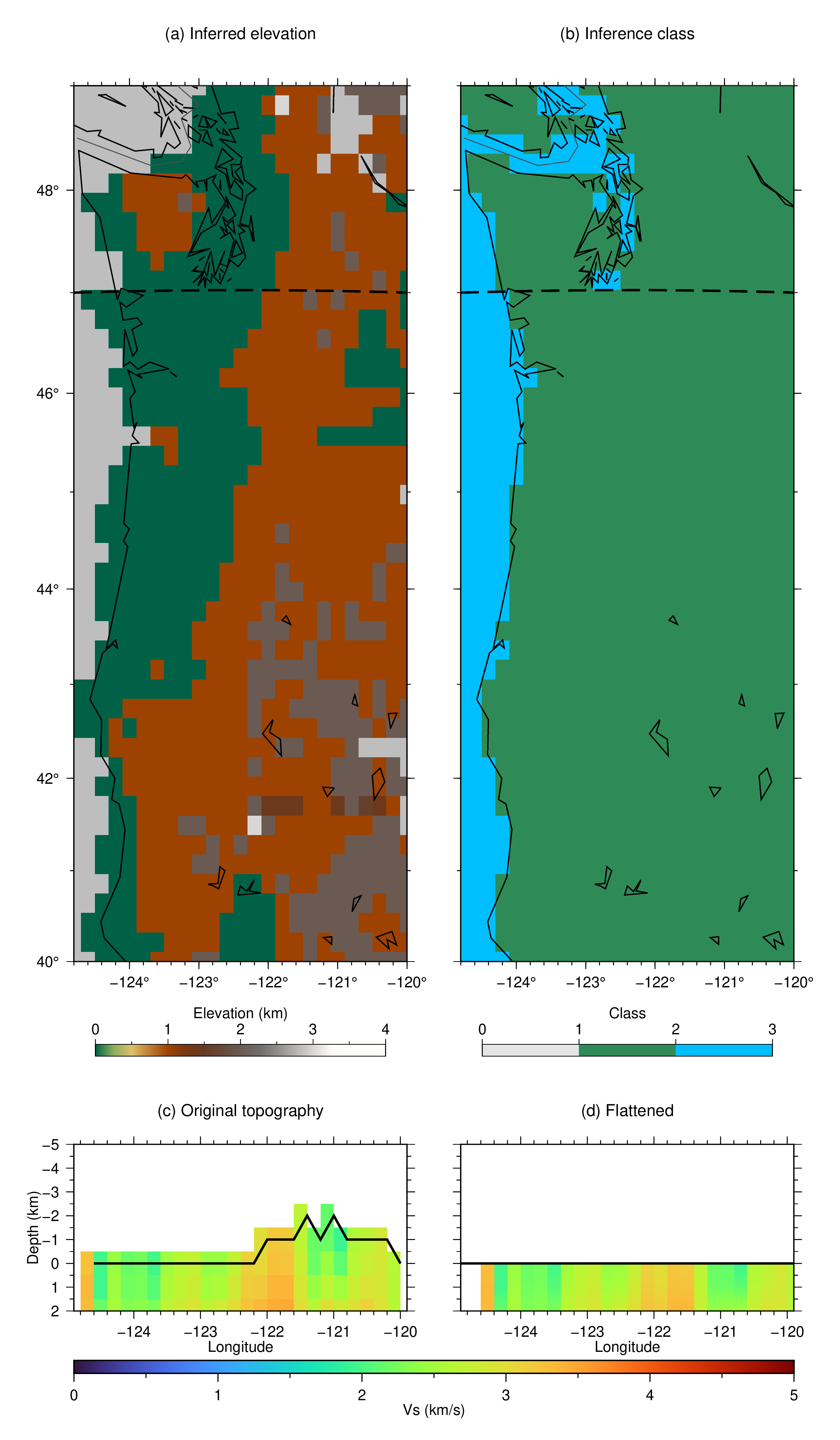
The diagnostics figure contains the inferred elevation, inference classes, the original latitude = 47 N section, and the flattened section. Class 0 marks unresolved columns outside the model coverage, class 1 marks land, and class 2 would mark a seafloor inferred from water values.

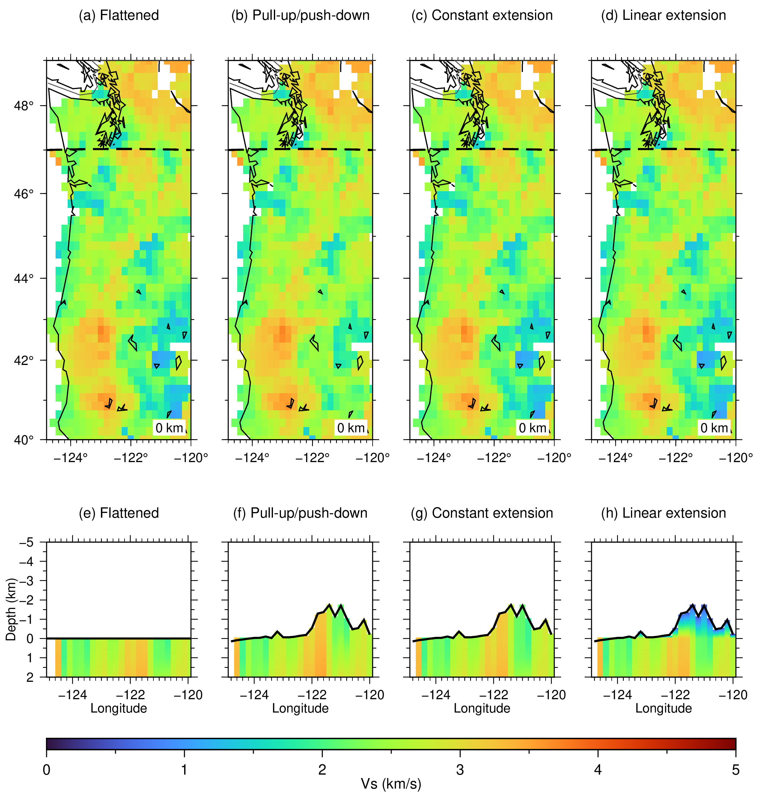
The methods figure compares the flattened baseline with:

• -Oa+t -Mp: pull-up/push-down construction

• -Oa+t -Me: constant one-dimensional construction

• -Oa+t -Ml -LVs/0.5: linear construction to 0.5 km/s at the land surface

The top row shows Vs at zero depth. The bottom row shows latitude = 47 N sections from 5 km elevation to 2 km depth. Dashed lines on the maps mark the section location, and solid lines on the sections mark the applied surface.

Run:

./ex06_ant_rf_gap_filling.sh

Intermediate NetCDF models are removed when the script exits. The script creates:

• ex06_ant_rf_gap_filling_diagnostics.png and ex06_ant_rf_gap_filling_diagnostics.pdf

• ex06_ant_rf_gap_filling_methods.png and ex06_ant_rf_gap_filling_methods.pdf

Figures

Downloads

• ex06_ant_rf_gap_filling.sh

• ex06_ant_rf_gap_filling_diagnostics.pdf

• ex06_ant_rf_gap_filling_methods.pdf